Excel Pivot Tables are sometimes a mystery to users of Excel. In this example I am going to show you how to add a percentage (%) column into a pivot table. This column will calculate that rows percentage of the grand total.

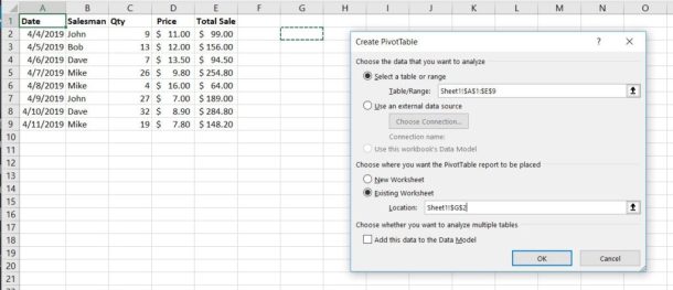
We will start with some sample raw data. In the worksheet above we have order information by a few salesman. We are going to start by creating a simple pivot table summarizing total sales by salesman. To create the pivot table click into any cell in the table (A1 for example). Next click the INSERT menu at the top of Excel. Next, click the PIVOT TABLE icon. This will bring up the below popup box. We are going to select to place the pivot table on the existing worksheet to the right of the table data.
From the Pivot Table Fields pane on the right hand side of Excel choose the checkbox next to Salesman and Total Sale. Next, confirm that the Salesman field is in the Rows box and that “Sum of Total Sale” is in the Values box in the bottom right. Your table should look like the below screen shot.

Format the pivot table column as currency
Just to keep the numbers looking neat and clean I am going to adjust the field properties to format the Total Sale column as Currency. To format the Total Sale column you can right click the column heading in the pivot table and choose Value Field Settings from the menu.

On the Value Field Settings box click the Number Format button in the bottom left of the screen as shown below.

This will bring up the Format Cells box. You should select the Currency option to display this column of data using the currency format.

When formatted your pivot table will now look like the below screen shot. Although this is not necessary, I like to get in the habit of making the data look as easily readable as possible.

Add the Percentage Column
To add a column to our pivot table that shows the percentages of total sales for each salesman we need to click and drag a second copy of the Total Sale column from the field list down to the Values section. It will look like the below screen shot.

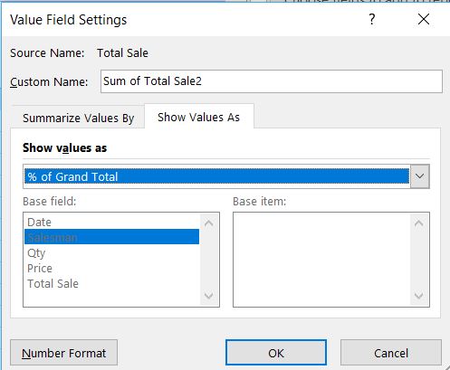
Next, we need to adjust the display of this second Sum of Total Sale column to show the percentage of grand total rather than another sum of the sales numbers. To do this, click the small triangle next to the field name in the Values box to show a menu. Choose the Value Field Settings to show the popup box where we will adjust the display of this field. Select the Show Values As tab. Next select the “Show values as” drop down box and choose “% of Grand Total” as shown below. After that you can click the OK button. The field/column will now be shown as percentages.
If all of the above steps were followed you should now have a Excel Pivot Table that has Salesman, Total Sales and Percentages as shown below.

Please post any questions or comments below. For more of my Excel Tips and Tricks.
[…] How to add a percentage column in a pivot table. – Working with pivot tables is very important for most jobs that require Excel skills. Learn how to customize a column in a pivot table. […]